This document describes a framework which was developed to test DM Stack shape measurement algorithms, as well as to compare algorithm configurations. It can be used with any algorithm housed in a measurement “plugin” as defined by the lsst.meas.base package. The plugin must produce a result which can be used to calculate galaxy ellipticity.
The algorithms tested in this document are in the meas_modelfit package, which houses both the CModel algorithm – used to measure galaxy shapes) and the ShapeletPsfApprox Algorithm (SPA) – used to create a parameterized model of the PSF (point spread function). Our goal was to run both PSF approximation and shape measurement on large numbers of simulated galaxies with known shear and PSF distortions, and to compare the shear measurements produced by diffent configurations of these algorithms.
We hope in the future to test a variety of shape algorithms, including future versions of CModel and SPA. The work described here is more of interest for the test techniques developed than for any particular result.
Techniques used in this simulations
Galaxy Shear Experiments Scripts
The framework for running these tests can be found in the repository https://github.com/lsst-dm/galaxy_shear_experiments. The README in this repository contains instructions for running this code.
Python scripts were used to automate the production of simulation images, the running of the measurement algorithm, and the analysis of the measured shear. The scripts allow single process mode, a parallel process mode on multiple core machines, and batch processing with a system such as the SLAC Batch Farm.
Test configurations and the PSF libraries actually used are not currently part of this repository, but will be added in the future. Scripts for parallel processing at SLAC will also be added as they are completed.
The great3sims scripts
The great3-public repository (https://github.com/barnabytprowe/great3-public) provided the scripts for creating catalogs of galaxies. This package draws galaxy parameters at random from a known distribution, and selects a PSF and applied shear for each galaxy. The scripts can output an “epoch catalog” and a yaml file for each value of applied shear. The epoch catalog has one row for each simulated galaxy, and gives the “true” galaxy characteristics and applied distortions. The yaml file and epoch catalog are in turn fed to GalSim, which creates a fits file of postage stamps of the galaxies.
Branch Setup:
The galaxy samples were selected using the great3sims “control/ground/constant” branch. This branch creates groups of galaxies in “subfields”, where all galaxies in a subfield have the same applied shear. The size of the postage stamps and the number of galaxies per subfield is configurable. Details of the configuration used are described with each test below.
Note that in all of our simulations, the galaxies are created as 90 degree rotated pairs to reduce shape noise.
One important modification to great3Sims was to sample the PSF for each galaxy from a PhoSim PSF Library (described below). Ordinarily, great3sims supplies the PSF specification to GalSim as a parameterized model. We suppled our own PSF libraries (a set of 67x67 pixel images at the LSST plate scale), using the GalSim InterpolatedImage type.
GalSim
See http://galsim-developers.github.io/GalSim for information about GalSim and how it is used. As discussed above, the great3Sims package supplies an epoch catalog for each subfield, as well as a matching yaml file which feeds the galaxy parameters to GalSim. The result is a gridded image of galaxies which can be used to make galaxy postage stamps.
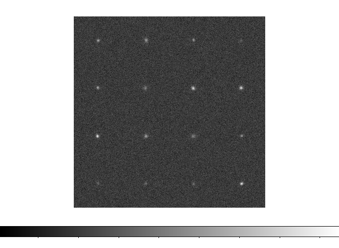
Figure 1 Galaxy images created by GalSim (this is a 4x4 galaxy subfield)
The epoch catalog is named epoch_catalog-nnn-m.fits, with nnn the ordinal number of the subfield, and m the epoch (always 0 in our tests). GalSim creates a matching image-nnn-m.fits with a 96x96 pixel image for each galaxy in the sample.
Creating the Phosim PSF Library:
PhoSim (version 3.4.2) is a ray tracing simulator which is used create images of galaxies and stars. This simulator has a description of the LSST telescope and camera, and will create simulated images with distortions due to variations in the atmosphere and optics. Please see https://confluence.lsstcorp.org/pages/viewpage.action?pageId=4129126 for a description of this software.
We used PhoSim to create stellar images scattered at random over the LSST focal plane. The LSST focal plane is divided into 21 rafts with 9 sensors per raft. To create a library of PSF images, 10000 positions were selected at random and PhoSim was instructed to create a stellar image at each position. After removing unusable stars (those which did not fall fully on any particular sensor, or which were close to another star), between 7000 and 8000 usable stellar images remained for each PSF library.
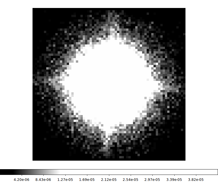
Figure 2 Psf created by PhoSim (67 x 67)
PSF libraries were created for “raw” seeing values of 0.5, 0.7, and 0.9 arcseconds through LSST filters f2 and f3 (r and i). The measured FWHM for these stellar images is actually somewhat worse after all the simulated distortions are applied.
Most of the tests during this cycle were run using the f2_0.7 or f3_0.7 libraries.
Doing Measurements:
The goal of the framework is to compare the results of some shape measurement plugin with the known shear values which stored in the epoch catalog. The algorithm must be housed in an lsst.meas.base measurement plugin, and it must produce either measure ellipticity, or some other value (e.g., second moments) which can be used to calculate ellipticity.
Our tests in this study were with the CModel algorithm with PSF modelling using ShapeletPsfApprox. The way in which these measurements are run is described in the galaxy_shear_experiments README.
Shear Bias Analysis:
We model shear bias as a combination of multiplicative bias (m) and additive bias (c)
gi = mi * g’i + ci
where g = (g1,g2) is the true shear and g’ = (g‘1, g‘2) is the measured shear.
To estimate these values, we perform a linear regression of applied shear vs. measured shear for both shear components.
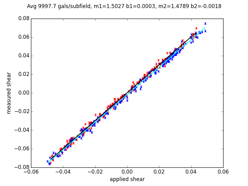
Figure 3 Graph of regression line fit to 200 subfield measurements
The individual points are for each of the 200 subfields: g1 values are shown in red, and g2 in blue. The g1 regression line is in black to make it visible on the plot.
In this example, the regression lines lie very close to each other, with the measured shear multiplicatively biased by about +50%. The intercepts deviate from zero by 7e-4 and 2e-4 respectively.
Of the 10000 galaxies in each subfield, a small percentage could not be measured due to fatal measurement errors.
Comparison of Shear Bias for Different Algorthms:
To see how different algorithms measure up, we plot their shear biases against each other. The plot shown below is a comparison of different parameterizations of the ShapeletPsfApprox(SPA) algorithm. Here, we compare a high order fit of the PSF (3773) against three lower order fits: SingleGaussian, DoubleGaussian, and Full. These are the predefined SPA parameterizations, and will be described in more detail later in this document.
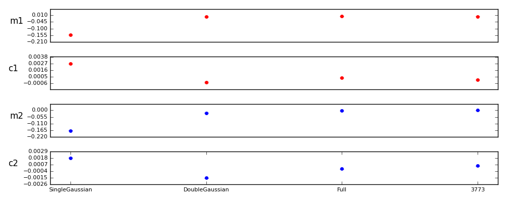
Figure 4 Comparison of shear bias for different algorithms
Note that the errorbars are shown in this graph, but are very small compared to the range of shear biases produced by these algorithms.
How errors were determined:
The errors in the shape bias were based on the difference between the measured and applied shear in each subfield. We calculated our errors in two ways. One was to use error estimators from each subfield to analytically determine the errors in the shear bias values. The other was to use a bootstrap technique to see how the regression values actually varied within resampled distributions.
In our test, we ran only one simulation for each test. Running 10 or even 20 samples of the same size and measuring the variation between samples would have been a useful technique for more accurately estimating the errors, and should be done in the future.
1. Calculated Errors
If (e1,e2) is the measure of the galaxy ellipticity and (g1,g2) is the applied shear, the deviation of (e1-g1,e2-g2) from (0,0) is a measure of the error. Of course, this measurement is dominated by shape noise, so we average over an subfields which contain large number of galaxies with the same applied shear.
Since the regression to determine m1, c1, m2 and c2 uses as its data the (e1avg, e2avg) vs. (g1, g2), we can use the errors in e1avg and e2avg to determine the errors in the regression values. See William H. Press, Numerical Recipes, 3rd edition, section 15.2 for a description of this calculation.
2. Bootstrap estimation
We did not entirely trust the approach under (1), so we used bootstrap resampling to produce different resampled populations of galaxies from our single set of 2 million galaxies. This allowed us to do the shear bias calculation multiple times and observe the variation in the shear parameters on these different populations. The great3sims subfields are actually 5000 galaxy pairs, not 10000 independent galaxies, so we actually resampled in pairs.
The bootstrap method consistently gives an error which is larger than the analytic approach by a factor of 2.1-2.3.
Since the ratio of the two was roughly constant and the calculated error is easier to get, we uniformly took as our error the calculated error multiplied by 2.2.
3. Error estimation with 10 realizations
10 runs of 2 million galaxies were run
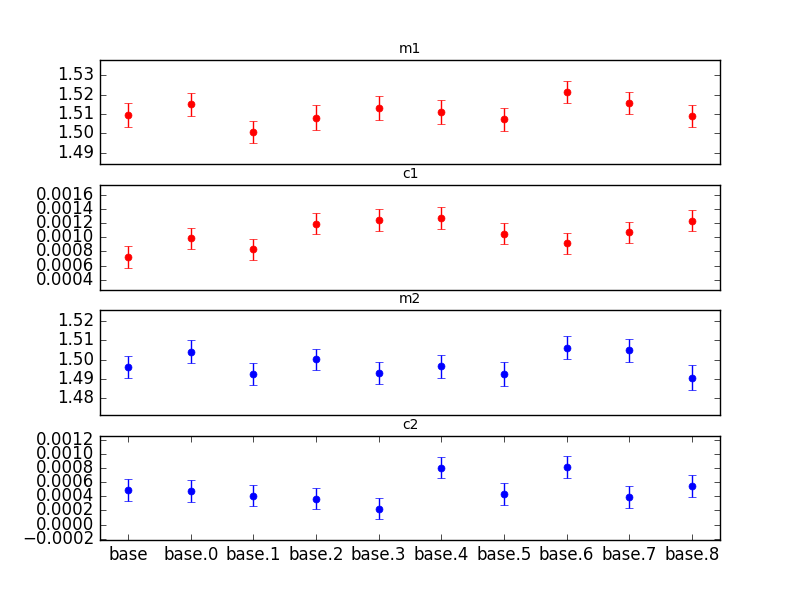
Figure 5 Comparison of 10 realizations of the great3sims test
Here are the statistics for the 10 runs. The values shown in parentheses are the standard deviations after calibrating the measurement to a slope of 1.0.
M1: 1.51109 +- 0.00562 (3.72e-3) range: 0.02061
B1: 0.00105 +- 0.00019 (1.25e-4) range: 0.00055
M2: 1.49777 +- 0.00574 (3.83e-3) range: 0.01560
B2: 0.00049 +- 0.00019 (1.24e-4) range: 0.00059
Testing Parameterizations of ShapeletPsfApprox
These tests were done under issues DM-1136 and DM-4214. To assess computational demands, we tested ShapeletPsfApprox (SPA) to find out how low the SPA fits orders can be without substantially affecting the quality of the PSF estimate. SPA is a four component “multi-shapelet function” model of the PSF, where the four components (from narrowest to broadest) are named “inner”, “primary”, “wings”, and “outer”. An SPA model is designated in this document with four numbers: for example, 1234 means inner order = 1, primary order = 2, wings order = 3, and outer order = 4.
In our earlier graph, SingleGaussian is -0–, Double Gaussian is -00-, and Full is 0440. (‘-‘ means that no value was fit for the component).
Test setup
Subfields: 100x100 (10000 galaxies in 5000 pairs). A total of 200 subfields for each test, with g1 and g2 selected as in the great3sims control/ground/constant branch.
PSF: filter f2 (r) and “raw seeing” 0.7 arcsecs. Single PSF selected from f2_0.7 PhoSim library.
Error estimation increased by multiplying the calculated error by 2.2. This correction was indicated by bootstrap tests.
Finding “best” parameterization for ShapeletPsfApprox
Comparing parameterizations is a little tricky, as the effects of the parameters are not independent of each other. To make this comparison more tractable, I’ve chose to take slices through the parameter space, relying to some extent on the previous experience that the “primary” parameter has the biggest effect, followed by the “wings”. The “inner” and “outer” seem to have less of an effect.
The first trial was to compare parameterizations of the form 0nn0, where n=2,3,4,5. The 3773 parameterization is shown for reference.
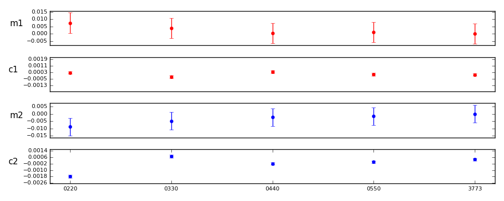
Figure 6 Parameterizations of the form 0nn0.
	  m1diff  sigmas  c1diff  sigmas  m2diff  sigmas  c2diff  sigmas
0220:	  0.0074  0.7601  0.0002  1.0268 -0.0087 -1.0127 -0.0021 -8.8106
0330:	  0.0038  0.3872 -0.0003 -1.1219 -0.0048 -0.5575  0.0004  1.6602
0440:	  0.0004  0.0382  0.0003  1.4533 -0.0022 -0.2608 -0.0005 -2.1926
0550:	  0.0010  0.0982  0.0000  0.1076 -0.0015 -0.1784 -0.0003 -1.2746
3773:	  0.0000  0.0000  0.0000  0.0000  0.0000  0.0000  0.0000  0.0000

Control value 3773 errs: m1 0.0069 c1 0.0002 m2 0.0061 c2 0.0002
The results appear to get better up to 0550. However, none of the models above 0330 differ from the 3773 model are different at the 3 sigma level.
However, note the similar comparisons with inner and outer set to 2 or 3. The primary and wings settings seem to settle by order 4 with higher order in the inner and outer components.
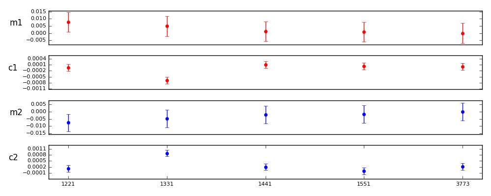
Figure 7 Parameterizations of the form 1nn1.
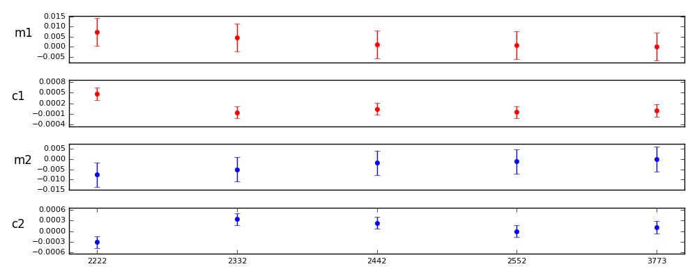
Figure 8 Parameterizations of the form 2nn2.

Figure 9 Parameterizations of the form 3nn3.
Here is a full set of comparisons against 3773 where primary and wings are the same, and inner and outer are the same. They suggest that order 3 may be nearly as good as the higher orders, with improvement in the PSF modeling appearing to max out between order 3 and 4.
	  m1diff  sigmas  c1diff  sigmas  m2diff  sigmas  c2diff  sigmas
Full:	  0.0004  0.0382  0.0003  1.4533 -0.0022 -0.2608 -0.0005 -2.1926
0330:	  0.0038  0.3872 -0.0003 -1.1219 -0.0048 -0.5575  0.0004  1.6602
0440:	  0.0004  0.0382  0.0003  1.4533 -0.0022 -0.2608 -0.0005 -2.1926
0550:	  0.0010  0.0982  0.0000  0.1076 -0.0015 -0.1784 -0.0003 -1.2746

1221:	  0.0077  0.7915 -0.0000 -0.1590 -0.0077 -0.8944 -0.0001 -0.4388
1331:	  0.0049  0.5013 -0.0007 -2.8448 -0.0047 -0.5534  0.0007  2.8550
1441:	  0.0013  0.1303  0.0001  0.4668 -0.0020 -0.2282 -0.0000 -0.0628
1551:	  0.0009  0.0942  0.0000  0.0970 -0.0017 -0.1954 -0.0002 -0.9167

2222:	  0.0073  0.7484  0.0005  1.9614 -0.0077 -0.8990 -0.0004 -1.7788
2332:	  0.0046  0.4727 -0.0001 -0.2355 -0.0051 -0.5953  0.0002  0.9511
2442:	  0.0010  0.1047  0.0000  0.1875 -0.0018 -0.2080  0.0001  0.5331
2552:	  0.0008  0.0786 -0.0000 -0.1917 -0.0011 -0.1288 -0.0001 -0.4570

3223:	  0.0076  0.7807 -0.0006 -2.4710 -0.0078 -0.9141 -0.0002 -0.8352
3333:	  0.0053  0.5380  0.0002  0.7282 -0.0050 -0.5867 -0.0000 -0.0741
3443:	  0.0006  0.0656  0.0002  0.8126 -0.0018 -0.2075 -0.0002 -0.7979
3553:	  0.0001  0.0114  0.0000  0.0238 -0.0014 -0.1600 -0.0001 -0.3764

Control value = 3773, errors: m1 0.0031 c1 0.0001 m2 0.0028 c2 0.0001
Conclusion:
The tests clearly favor order 3 parameterizations or higher, with 3333 within the errorbars of 3773. It also appears that it is important to have at least order 2 in the inner and outer components.
It is obvious that a lot depends on our error assumptions. Most of the parameterizations at order 3 or higher do not appear to be significantly different, but would be without the 2.2x error multiplier. In future studies, we will run more simulations to improve our understanding of the errors.
Testing CModel Configurations
Our earliest tests were tests of CModel configurations. For these tests, the SPA was held at its defaults, and Cmodel was run through a range of its configuration values.
We reproduce here a couple of results having to do with the size of the measurement area used by the CModel algorithm.
These tests were also useful in assessing how many galaxies would be needed to see significant differences. As a result of these these tests, we decided to move our tests from single host, multi-core machines at Davis to the computing farm at SLAC, as larger galaxy populations were seen to be needed.
Test setup
Subfields: 32x32 (1024) galaxies/subfield, or 512 pairs. The applied shear was varied in 6 steps from .0001 to .05. The shear angle was random from 0-360 for each of subfield. While this subfield arrangement has only specific values of g = sqrt(g1*g1 + g2*g2), it actually has a very uniform selection of g1 and g2.
Tests varied in size from as few as 128 subfields to as many as 2048. Initial tests were done with a small number of galaxies, but the number of subfields was increased until we were able to clearly see the results.
PSF: filter f3 (i) and “raw seeing” 0.7 arcsecs. Random PSF selected for each galaxy.
Error estimation indicated by using the “calculated” regression errors. No bootstraps were run.
Test Descriptions:
Initially, the test was done with 128 subfields at 6 shear values (.0001, .01, .02, .03, .04, .06), for a total of 786,432 galaxies.
When these intial tests were not sensitive enough, tests of 1024 subfields and later 2048 subfields were tried (up to 12 million galaxies).
The results of the earlier tests were published with the Summer 2015 issues, DM-3375 and DM-1135. These tests showed obvious trends, but did not have large enough galaxy samples to display significant pair-wise differences.
The results shown below were done for DM-3983, which was a retest with 1024 subfields for each of the 6 shear values, or about 6 million galaxies total. Because of time constraints, only a few of the critical nGrowFootprint and stampsize values were retested.
nGrowFootprint Test:
In this test, the nGrowFootprint configuration of CModel was varied from 0 to 10. The meas_base measurement algorithm starts with a galaxy “footprint”, which is derived from the set of pixels above the detection threshold. This default footprint is used when nGrowFootprint = 0. For positive values of nGrowFootprint, the measurement area is expanded in all directions by that amount. Values of nGrowFootprint which would extend the footprint beyond the bounds of the original postage stamp are not allowed.
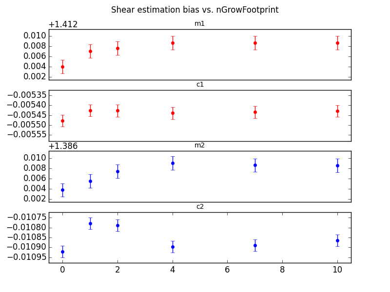
Figure 10 nGrowFootprint vs. shear bias
Stampsize Test:
In this test, the measurement footprint was always a square, regardless of the contours of the actual galaxy. The same GalSim images were used in all these tests, but the stampsize was decreased in software by trimming the postage stamps provided to the CModel algorithm. The original galaxy postage stamps created by GalSim were 96x96 at the LSST plate scale. Test were run from 20x20 to 96x96. The values for 20, 40, and 64 are shown below.
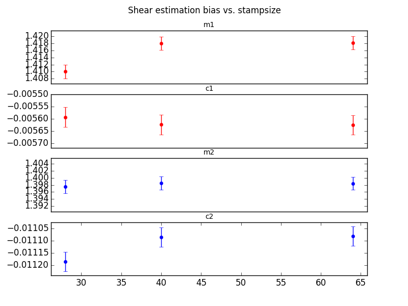
Figure 11 stampsize vs. shear bias
Conclusion:
We were able to show significant differences in measured shear values, both by allowing the footprint to expand, and by forceably truncating the postage stage for each galaxy.
The original 768K galaxy sample was not large enough to show these differences. A much larger study of 6 million galaxies was adequate.
We did not pursue just how large the galaxy population had to be, or exactly what values of these two tests were optimal.